Reporting and visualization
Source:vignettes/reporting-and-visualization.Rmd
reporting-and-visualization.RmdGoal
This guide focuses on communication-ready output workflows:
- Format fit results for markdown and HTML reports.
- Export fit tables to Word.
- Visualize single-model and multi-model fit summaries with
plot_model_fit(). - Use
plot_factor_loadings()as a complementary structural view.
Setup
library(psymetrics)
library(lavaan)

model <- '
  visual  =~ x1 + x2 + x3
  textual =~ x4 + x5 + x6
  speed   =~ x7 + x8 + x9
'

fit_mlr <- cfa(
  model,
  data = HolzingerSwineford1939,
  estimator = "MLR"
)
fit_ulsm <- cfa(
  model,
  data = HolzingerSwineford1939,
  estimator = "ULSM"
)
fit_mlr_multi <- cfa(
  model,
  data = HolzingerSwineford1939,
  estimator = "MLR",
  test = c("satorra.bentler", "mean.var.adjusted")
)

single_fit <- model_fit(fit_mlr)
compared_fits <- compare_model_fit(MLR = fit_mlr, ULSM = fit_ulsm)
single_fit_multi <- model_fit(fit_mlr_multi, standard_test = TRUE)
Format results for markdown, HTML, and auto output
To request markdown output explicitly:
format_results(compared_fits, output = "markdown")|MODEL | NOBS | ESTIMATOR | NPAR | Chi2(24) | p (Chi2) | CFI | TLI | RMSEA | RMSEA CI | SRMR |
|:-----|:----:|:---------:|:----:|:--------:|:--------:|:-----:|:-----:|:-----:|:--------------:|:-----:|
|MLR | 301 | MLR | 21 | 87.13 | < .001 | 0.925 | 0.888 | 0.093 | [0.073, 0.115] | 0.065 |
|ULSM | 301 | ULSM | 21 | 90.60 | < .001 | 0.931 | 0.897 | 0.096 | [0.073, 0.120] | 0.059 |In an HTML report or pkgdown article, the same object can render directly as a formatted table:
| MODEL | NOBS | ESTIMATOR | NPAR | Chi2(24) | p (Chi2) | CFI | TLI | RMSEA | RMSEA CI | SRMR |
|---|---|---|---|---|---|---|---|---|---|---|
| MLR | 301 | MLR | 21 | 87.13 | < .001 | 0.925 | 0.888 | 0.093 | [0.073, 0.115] | 0.065 |
| ULSM | 301 | ULSM | 21 | 90.60 | < .001 | 0.931 | 0.897 | 0.096 | [0.073, 0.120] | 0.059 |
By default, format_results(compared_fits) uses
output = "auto" and chooses markdown or HTML according to
the rendering context.
In HTML-capable contexts, you can also request HTML explicitly:
format_results(compared_fits, output = "html")| MODEL | NOBS | ESTIMATOR | NPAR | Chi2(24) | p (Chi2) | CFI | TLI | RMSEA | RMSEA CI | SRMR |
|---|---|---|---|---|---|---|---|---|---|---|
| MLR | 301 | MLR | 21 | 87.13 | < .001 | 0.925 | 0.888 | 0.093 | [0.073, 0.115] | 0.065 |
| ULSM | 301 | ULSM | 21 | 90.60 | < .001 | 0.931 | 0.897 | 0.096 | [0.073, 0.120] | 0.059 |
Export to Word
save_table(
  compared_fits,
  path = "model_fit.docx",
  orientation = "landscape"
)
Visualize a single fitted model
plot_model_fit() is the public plotting entrypoint for
model_fit() and compare_model_fit() objects.
For a one-row model_fit summary, the default style resolves
to the single-fit bullet chart.
plot_model_fit(single_fit)
Visualize a model comparison
For compare_model_fit() objects, the default plot is the
threshold-aware dot plot, which works well as a quick side-by-side
comparison.
plot_model_fit(compared_fits)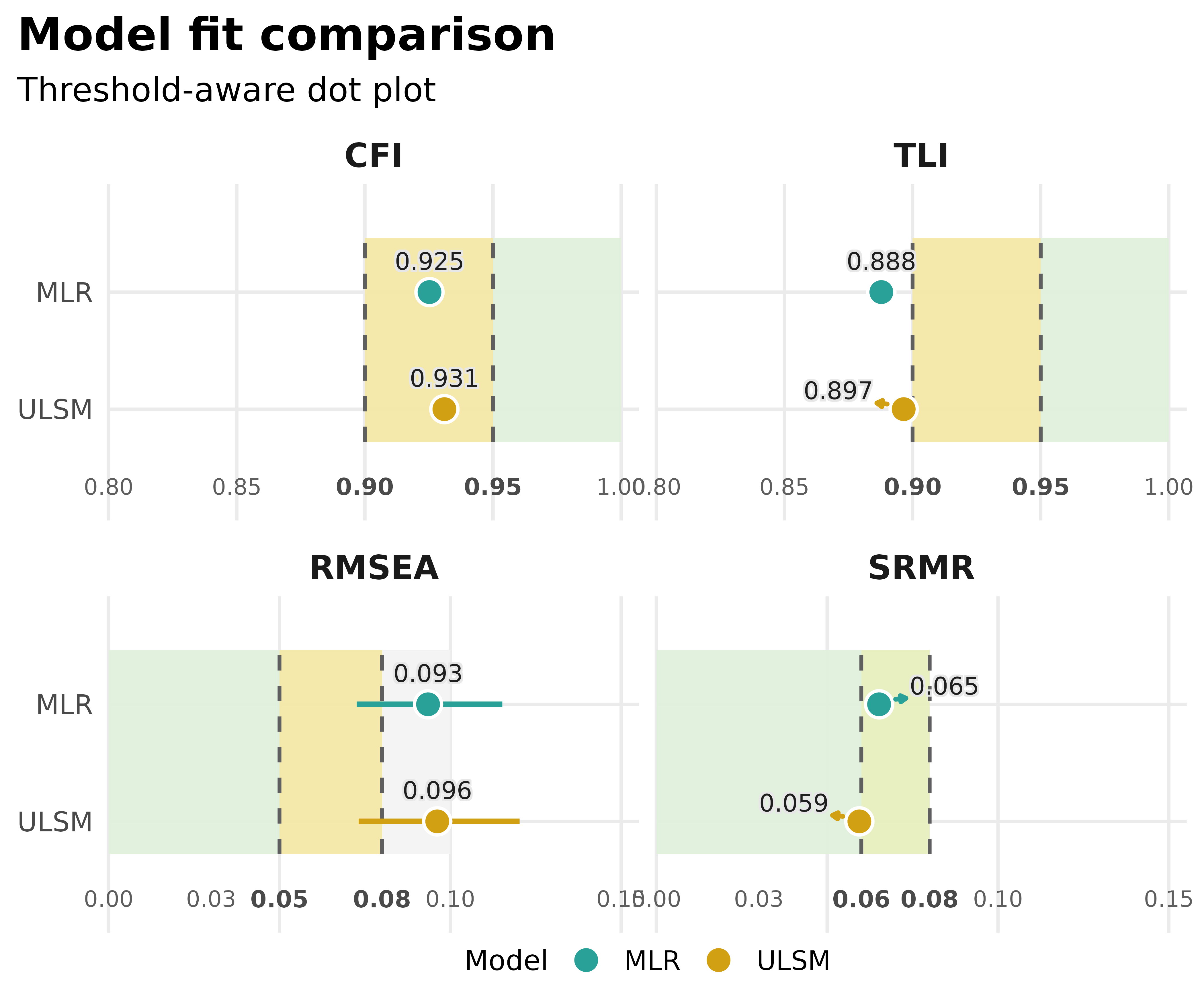
Try an alternative plot style
In v0.5.0, the supported plot styles are
default, bullet, dots,
bars, and heatmap. The article keeps to the
main workflow, while the plot_model_fit reference
documents the full argument surface and supported constraints.
plot_model_fit(compared_fits, type = "bars")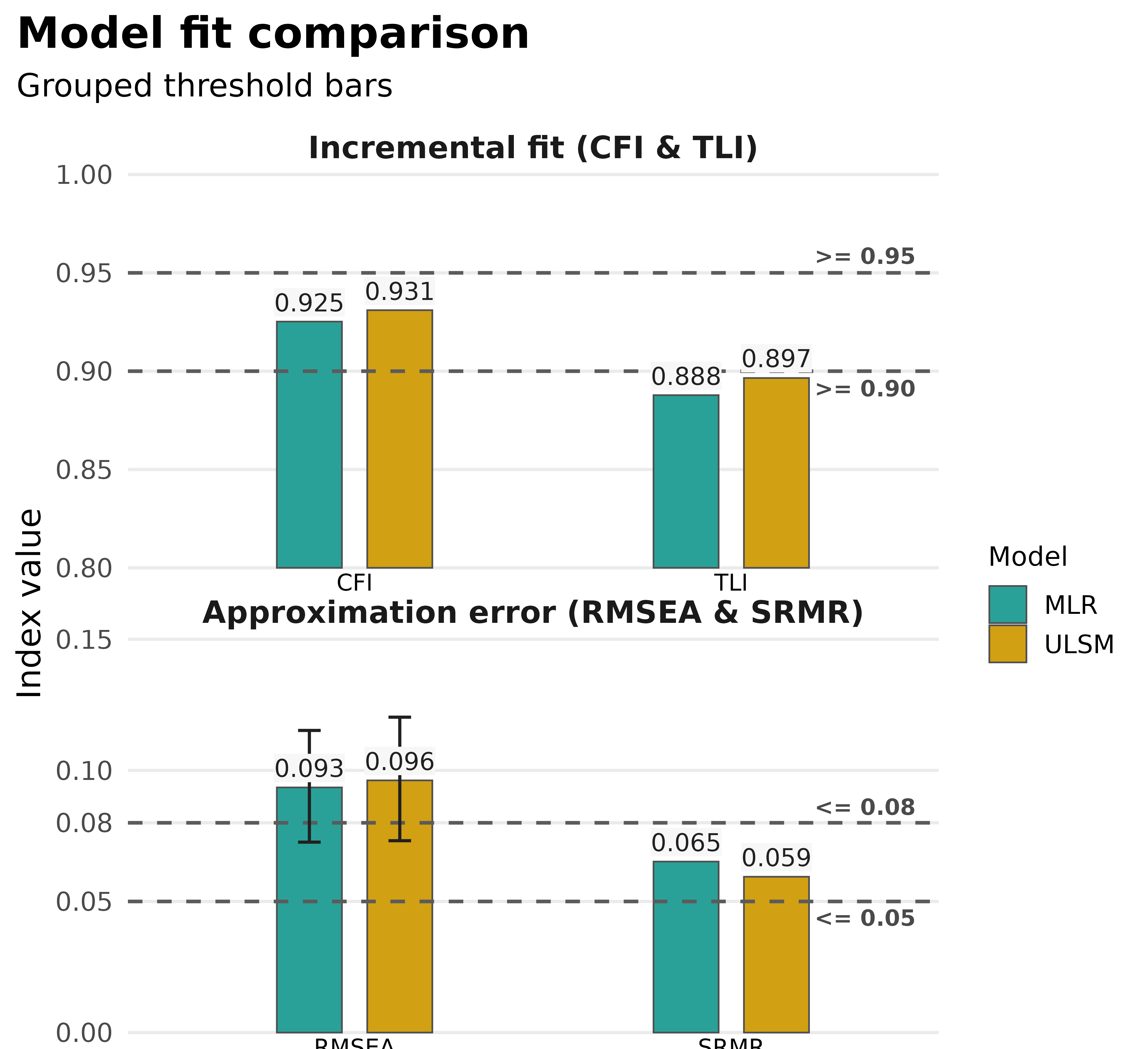
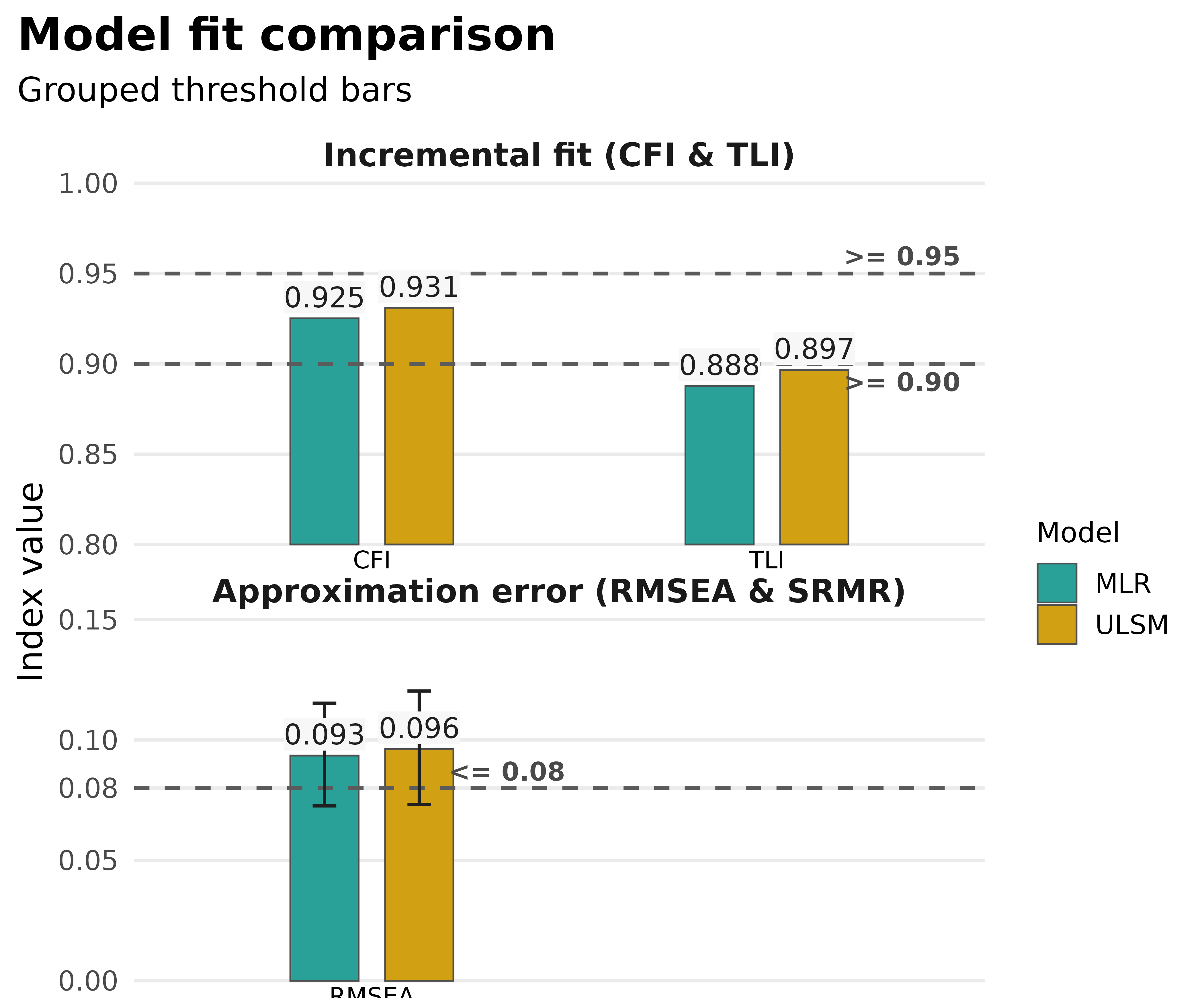
Focus on selected metrics
If you only want to communicate part of the fit summary, pass a
subset with metrics.
plot_model_fit(
  compared_fits,
  type = "bars",
  metrics = c("CFI", "TLI", "RMSEA")
)
Work with multiple test rows
When the fit object keeps both standard and non-standard test
summaries, plot_model_fit() can filter which rows to show
with test_mode. Here, standard_test = TRUE
keeps multiple rows in the model_fit() result, and
test_mode = "primary" reduces the view to the primary
non-standard summary.
plot_model_fit(single_fit_multi, test_mode = "primary")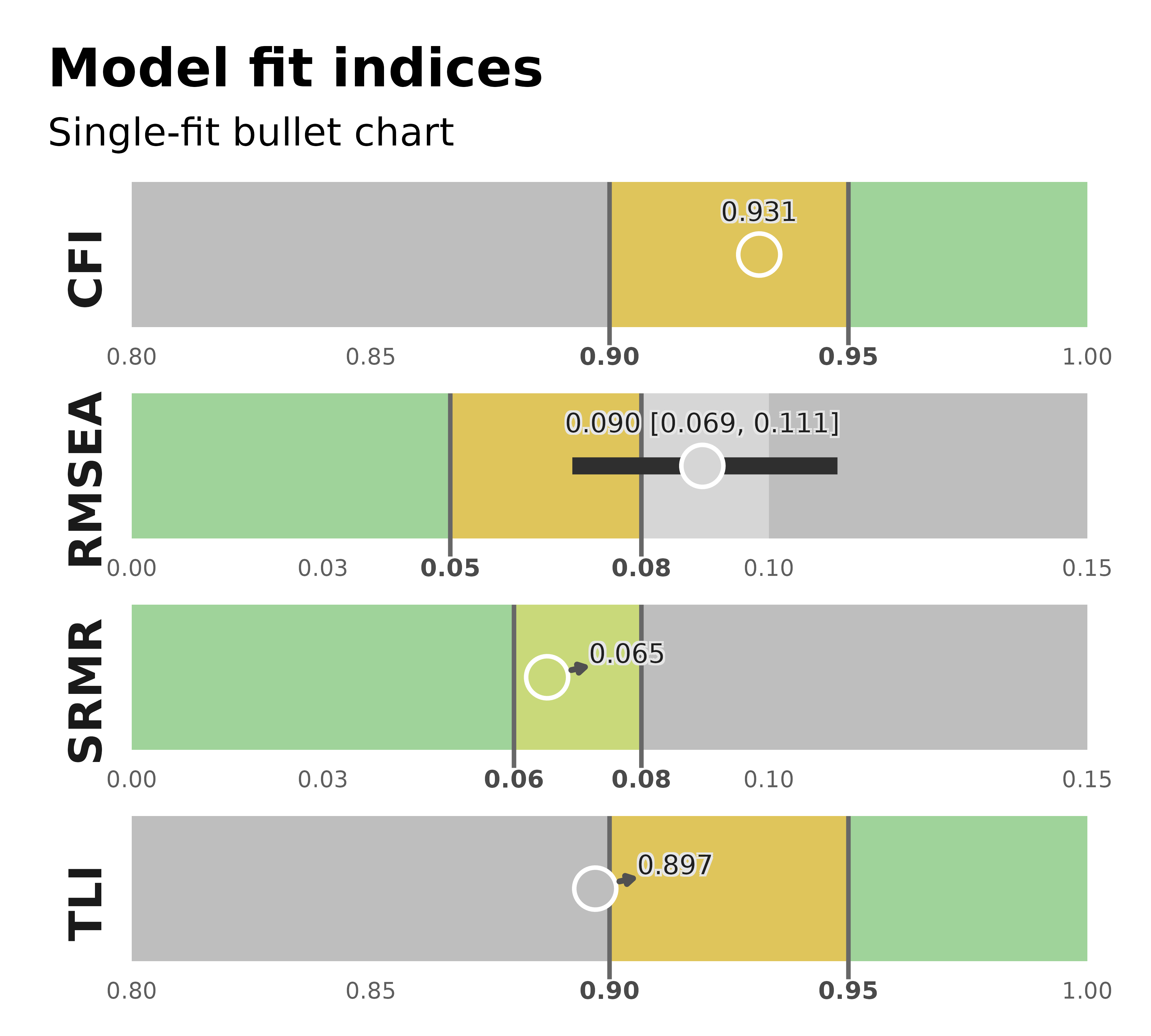
Visualize factor loadings as a complementary check
plot_model_fit() answers how well the model fits
overall. plot_factor_loadings() adds a complementary view
of the measurement structure after the fit summary looks acceptable.
plot_factor_loadings(fit_mlr)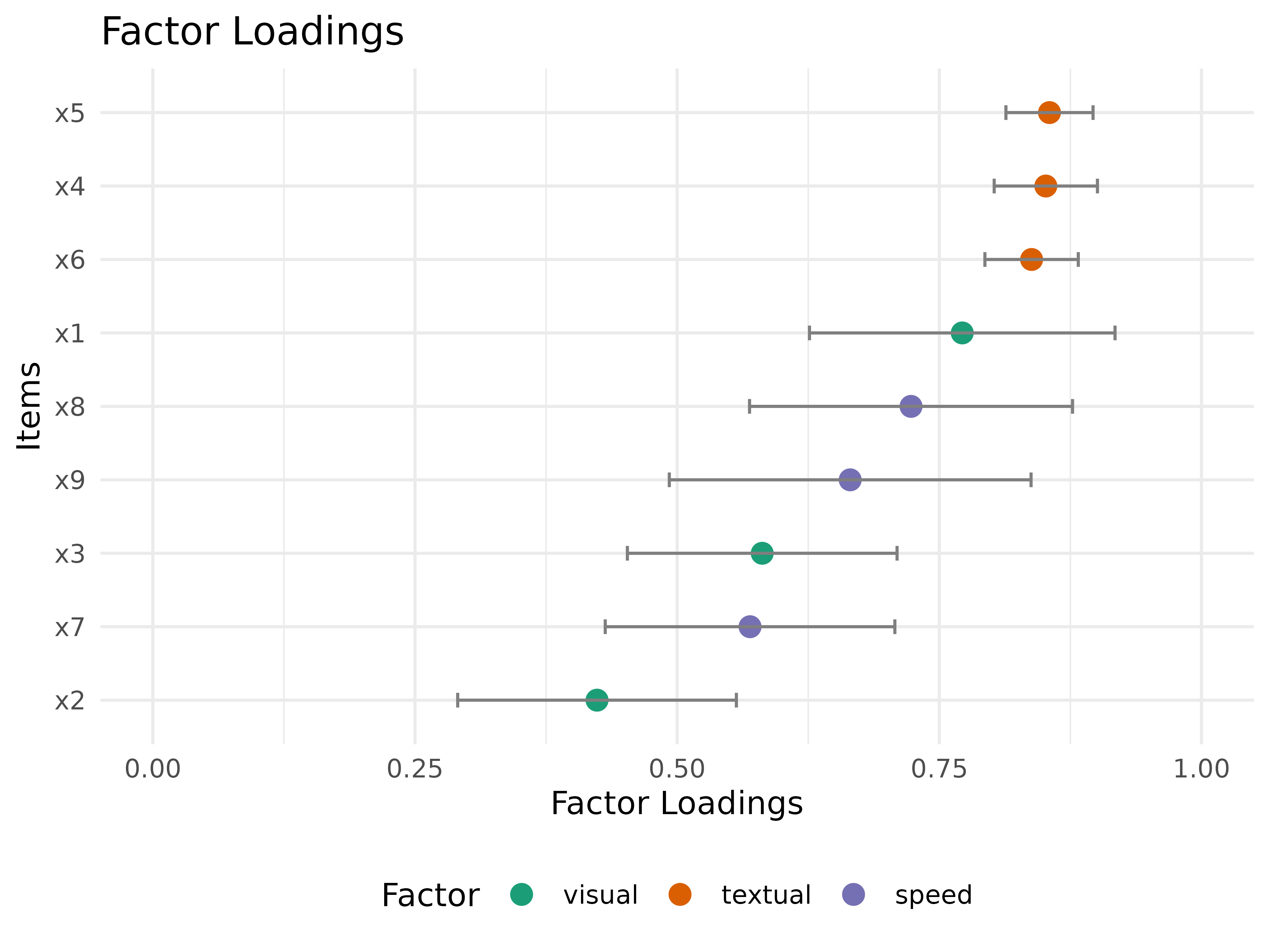
Practical notes
- Use
format_results()when you want the same fit object rendered in reports. - Use
save_table()when the output needs to go into a.docxworkflow. - Use
plot_model_fit()for the supportedCFI/TLI/RMSEA/SRMRworkflows inv0.5.0, and keep the reference page nearby for argument-level detail. - Use
plot_factor_loadings()after fit checking when you want to discuss item structure rather than overall fit.
Next steps
- Return to Get started with fit indices.
- Continue with SEM and parameter estimates.
- Explore the Reference for argument-level control.